Kernighan-Lin
Intro
In the last two posts, we discussed two random graph models that have community structure built in and applied the MAP to simplify the optimization problem. In this post we will discuss a heuristic to find optimal groups for the nodes of a network. The algorithm is discussed in the Karrer and Newman paper we talked about in the last post and it’s based (however not exactly the same) on an algorithm developed by Brian Kernighan (major contributor to the development Unix) and Shen Lin for graph partitioning. In this post we will discuss a naïve implementation and application to community detection of this algorithm.
Setup
I will be implementing this algorithm in python and the very first steps will be importing the right libraries
import graph_tool.all as gt
import numpy as np

import matplotlib.pyplot as plt
plt.style.use('ggplot')
Now let’s define a class to encapsulate all the variables and methods we will need for community detection
class Communities:
    """
    Class for dividing networks into communities
    """
    def __init__(self, graph, k, model='sbm'):
        """
        Initialize network with k communities according to a particular random graph model

        Args:
            graph (graph_tool.Graph): graph_tool graph object. Network to be partitioned into communities
            k (int): Number of communities to partition network into
            model (str, optional): Random graph model according to which the network will be partitioned. Defaults to 'sbm'.
        """
        self.graph = graph  # takes a graph_tool graph object
        self.num_groups = k  # number of groups to assign nodes to
        if model in ['sbm', 'dcsbm']:
            self.model = model
        else:
            raise ValueError('Invalid model. Choose from \'sbm\' or \'dcsbm\'')
        self.init_random_partition()  # randomly partition the network in to k groups
        self.curr_groups = self.partition()  # current group assignments
In the constructor I’ve declared several variables that are necessary on instantiation. The first three variables are passed by the constructor, the graph variable is the network we hope to partition into communities, the num_groups variable is the number of communities we are trying to find, and model is the random graph model we want to assume our network was generated from. We have discussed two related models: the Stochastic Block Model and the Degree Corrected Stochastic Block Model, depending on the model we choose we may (or may not) get different divisions of the network into communities.
The self.init_random_partition() line runs a method (which will be discussed below) that randomly assigns groups to nodes, we then generate a group assignment matrix by running self.partition() and store it in the curr_groups variable.
The first step in setting up the problem is to randomly assign nodes to group. This can be done quite simply using numpy and graph-tool
    def init_random_partition(self):
        """
        Randomly assigns groups to each node
        """
        partitions = self.graph.new_vertex_property('int')
        self.graph.vertex_properties['group'] = partitions

        for u in self.graph.iter_vertices():
            partitions[u] = np.random.randint(self.num_groups)
What this method does is create a new property for the nodes of our input network called “group”, it then assigns a random number between \(0\) and \(k-1\) (where \(k\) is the number of groups) to the property of each node.
Once we have assigned nodes to groups, we need a method that will generate the group assignment matrix (\(\Gamma\) in the previous derivations) based on the current assignments.
    def partition(self):
        """
        Generates group assignment matrix

        Returns:
            groups (numpy.ndarray): group assignment matrix of shape number of nodes by number of groups
        """
        groups = np.zeros(shape=(self.graph.num_vertices(),
                          self.num_groups), dtype=np.int32)

        labels = self.graph.vp.group.a
        for j in range(groups.shape[1]):
            for i in range(groups.shape[0]):
                groups[i, j] = 1 if j == labels[i] else 0

        return groups
This method simply returns a binary matrix where the columns represent groups, the rows represent nodes, and the entries tell whether a node is in a particular group or not based on the vertex property assigned in init_random_partition().
Lastly, before we get to the meat and potatoes of the problem, we need a way to calculate the log likelihood of our random graph model. This is simply just coding up the likelihood of the SBM or the DC-SBM.
    def sbm_likelihood(self):
        """
        Calculates the likelihood of the community structure according to the Stochastic Block Model

        Returns:
            float: Likelihood according to Stochastic Block Model
        """
        n_nodes = self.graph.num_vertices()

        nodes_in_grp = self.curr_groups.sum(axis=0)
        two_m = 2*self.graph.num_edges()

        edge_adj = self.curr_groups.T@(gt.adjacency(
            self.graph).todense())@self.curr_groups

        L = 0
        for r in range(edge_adj.shape[0]):
            for s in range(edge_adj.shape[1]):
                if(edge_adj[r, s] == 0):
                    L += 0
                else:
                    log_exp = np.log(edge_adj[r, s])-np.log(nodes_in_grp[r]*nodes_in_grp[s])
                    L += (edge_adj[r, s]*log_exp)

        return L
Detecting Communities
Karrer and Newman explain that the algorithm works by repeatedly moving nodes from one group to another and recording the log likelihood. We then select the node move that most increases (or least decreases) the log likelihood. This is done until every node is been moved exactly once and then repeated over several trials until we see that the log likelihood no longer increases. Let’s code this up
    def get_communities(self):
        """
        Performs Kernighan-Lin (https://ieeexplore-ieee-org.proxy.lib.umich.edu/document/6771089) like moves to find optimal
        community structure of network based on discussion by Karrer and Newman (https://arxiv.org/abs/1008.3926)

        Returns:
            list: best probability of each iteration of the algorithm
        """

        two_m = 2*self.graph.num_edges()
        n_nodes = self.graph.num_vertices()
        nodes = [i for i in range(n_nodes)]
        max_num_trials = 100

        if (self.model == 'sbm'):
            log_prob = self.sbm_likelihood
        else:
            log_prob = self.dcsbm_likelihood

        init_likelihood = log_prob()
        best_probs = [init_likelihood]

        for t in range(max_num_trials):
            unvisited = nodes.copy()
            t_best_config = np.zeros(shape=(n_nodes, n_nodes))
            max_probs = np.zeros(n_nodes)
            state = 0
            while(unvisited):
                probs = []
                for i in unvisited:
                    group_r = self.graph.vp.group[i]
                    curr_part = np.copy(self.curr_groups)
                    for group_s in range(self.num_groups):
                        if group_s != group_r:
                            self.graph.vp.group[i] = group_s
                            self.curr_groups = self.partition()
                            probs.append((log_prob(), i, group_s))

                            self.graph.vp.group[i] = group_r
                            self.curr_groups = np.copy(curr_part)

                max_prob = max(probs)
                max_probs[state] = max_prob[0]
                self.graph.vp.group[max_prob[1]] = max_prob[2]
                t_best_config[state] = self.graph.vp.group.a.copy()
                unvisited.remove(max_prob[1])
                state += 1
            if ((max_probs.max() - max(best_probs)) <= 0):
                return best_probs

            self.graph.vp.group.a = t_best_config[max_probs.argmax()].copy()
            best_probs.append(max_probs.max())

        return best_probs
The while loop ensures that in every trial, each node is only moved once, this is done by popping the node move that most increased the likelihood from the list of possible node moves (unvisited), when the list is empty, the loop stops. When iterating through unvisited we test each possible node move and store the node, the group to which we moved it, and the log likelihood. At the end, we accept the move associated with the highest log likelihood. We repeat this until we see that the log likelihood of any possible move is less than or equal to the highest log likelihood seen out of all the trials. These types of moves always ensure that the likelihood increases with every accepted move, so you should never see a decreasing likelihood.
All together our class looks like:
class Communities:
    """
    Class for dividing networks into communities
    """
    def __init__(self, graph, k, model='sbm'):
        """
        Initialize network with k communities according to a particular random graph model

        Args:
            graph (graph_tool.Graph): graph_tool graph object. Network to be partitioned into communities
            k (int): Number of communities to partition network into
            model (str, optional): Random graph model according to which the network will be partitioned. Defaults to 'sbm'.
        """
        self.graph = graph  # takes a graph_tool graph object
        self.num_groups = k  # number of groups to assign nodes to
        if model in ['sbm', 'dcsbm']:
            self.model = model
        else:
            raise ValueError('Invalid model. Choose from \'sbm\' or \'dcsbm\'')
        self.init_random_partition()  # randomly partition the network in to k groups
        self.curr_groups = self.partition()  # current group assignments

    def init_random_partition(self):
        """
        Randomly assigns groups to each node
        """
        partitions = self.graph.new_vertex_property('int')
        self.graph.vertex_properties['group'] = partitions

        for u in self.graph.iter_vertices():
            partitions[u] = np.random.randint(self.num_groups)

    def partition(self):
        """
        Generates group assignment matrix

        Returns:
            groups (numpy.ndarray): group assignment matrix of shape number of nodes by number of groups
        """
        groups = np.zeros(shape=(self.graph.num_vertices(),
                          self.num_groups), dtype=np.int32)

        labels = self.graph.vp.group.a
        for j in range(groups.shape[1]):
            for i in range(groups.shape[0]):
                groups[i, j] = 1 if j == labels[i] else 0

        return groups

    def sbm_likelihood(self):
        """
        Calculates the likelihood of the community structure according to the Stochastic Block Model

        Returns:
            float: Likelihood according to Stochastic Block Model
        """
        n_nodes = self.graph.num_vertices()

        nodes_in_grp = self.curr_groups.sum(axis=0)
        two_m = 2*self.graph.num_edges()

        edge_adj = self.curr_groups.T@(gt.adjacency(
            self.graph).todense())@self.curr_groups

        L = 0
        for r in range(edge_adj.shape[0]):
            for s in range(edge_adj.shape[1]):
                if(edge_adj[r, s] == 0):
                    L += 0
                else:
                    log_exp = np.log(edge_adj[r, s])-np.log(nodes_in_grp[r]*nodes_in_grp[s])
                    L += (edge_adj[r, s]*log_exp)

        return L


    def get_communities(self):
        """
        Performs Kernighan-Lin (https://ieeexplore-ieee-org.proxy.lib.umich.edu/document/6771089) like moves to find optimal
        community structure of network based on discussion by Karrer and Newman (https://arxiv.org/abs/1008.3926)

        Returns:
            list: best probability of each iteration of the algorithm
        """

        two_m = 2*self.graph.num_edges()
        n_nodes = self.graph.num_vertices()
        nodes = [i for i in range(n_nodes)]
        max_num_trials = 100

        if (self.model == 'sbm'):
            log_prob = self.sbm_likelihood
        else:
            log_prob = self.dcsbm_likelihood

        init_likelihood = log_prob()
        best_probs = [init_likelihood]

        for t in range(max_num_trials):
            unvisited = nodes.copy()
            t_best_config = np.zeros(shape=(n_nodes, n_nodes))
            max_probs = np.zeros(n_nodes)
            state = 0
            while(unvisited):
                probs = []
                for i in unvisited:
                    group_r = self.graph.vp.group[i]
                    curr_part = np.copy(self.curr_groups)
                    for group_s in range(self.num_groups):
                        if group_s != group_r:
                            self.graph.vp.group[i] = group_s
                            self.curr_groups = self.partition()
                            probs.append((log_prob(), i, group_s))

                            self.graph.vp.group[i] = group_r
                            self.curr_groups = np.copy(curr_part)

                max_prob = max(probs)
                max_probs[state] = max_prob[0]
                self.graph.vp.group[max_prob[1]] = max_prob[2]
                t_best_config[state] = self.graph.vp.group.a.copy()
                unvisited.remove(max_prob[1])
                state += 1
            if ((max_probs.max() - max(best_probs)) <= 0):
                return best_probs

            self.graph.vp.group.a = t_best_config[max_probs.argmax()].copy()
            best_probs.append(max_probs.max())

        return best_probs
The full code, including the degree corrected likelihood implementation can be accessed here
Testing the Code
Simple Network
Let’s begin by loading up a simple network for us to test this algorithm on (included in the github repo).
test_graph = gt.load_graph('test_block_graph.graphml')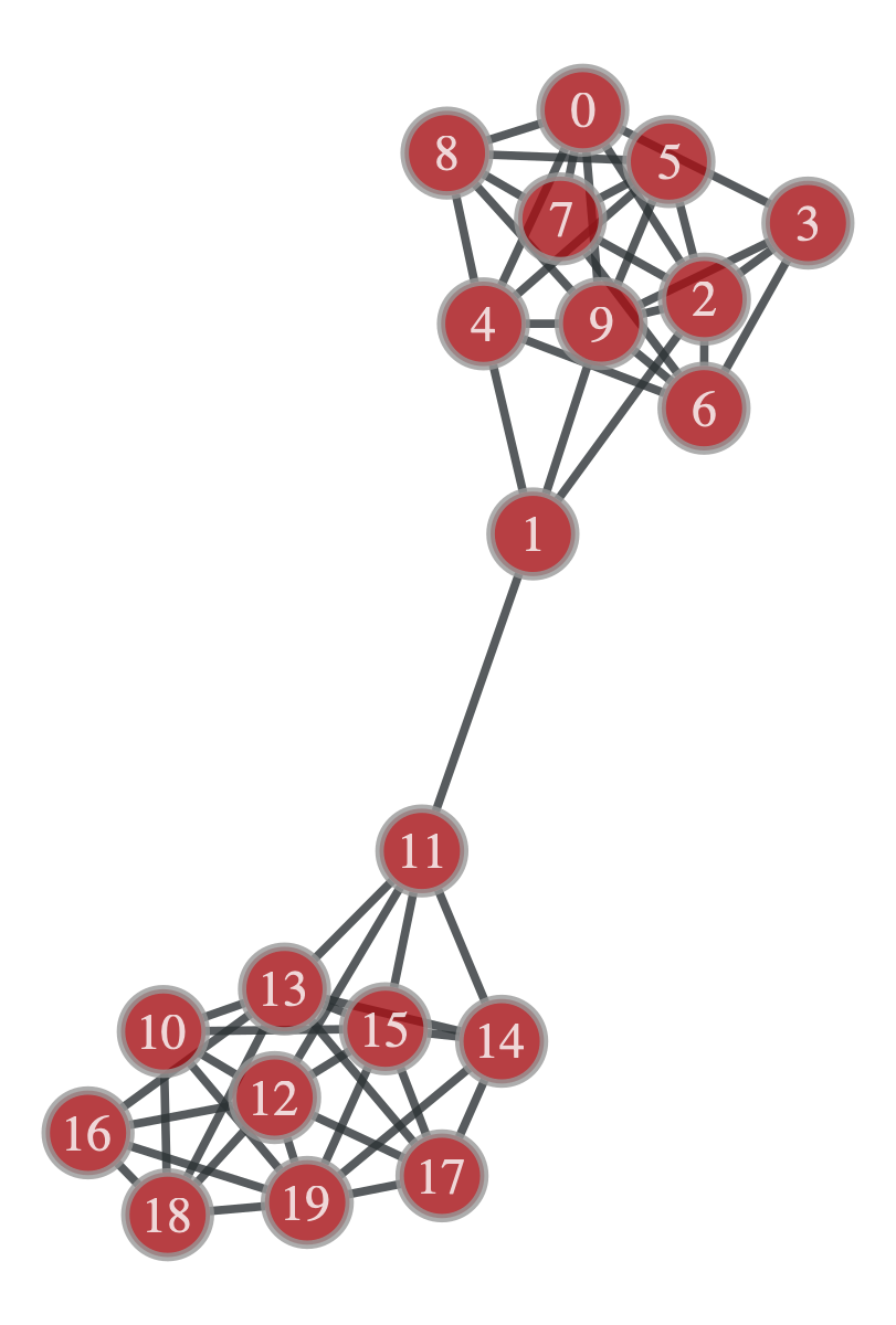 The above network has got 20 nodes with two very obvious communities. Let’s create a
 Communities object and test how our algorithm does.
test_sbm = Communities(test_graph, 2, 'sbm')With the 'sbm' argument, we are indicating that we would like the communities to be determined according to the stochastic block model. So now we run the get_communities() method and inspect the result
sbm_probs = test_sbm.get_communities()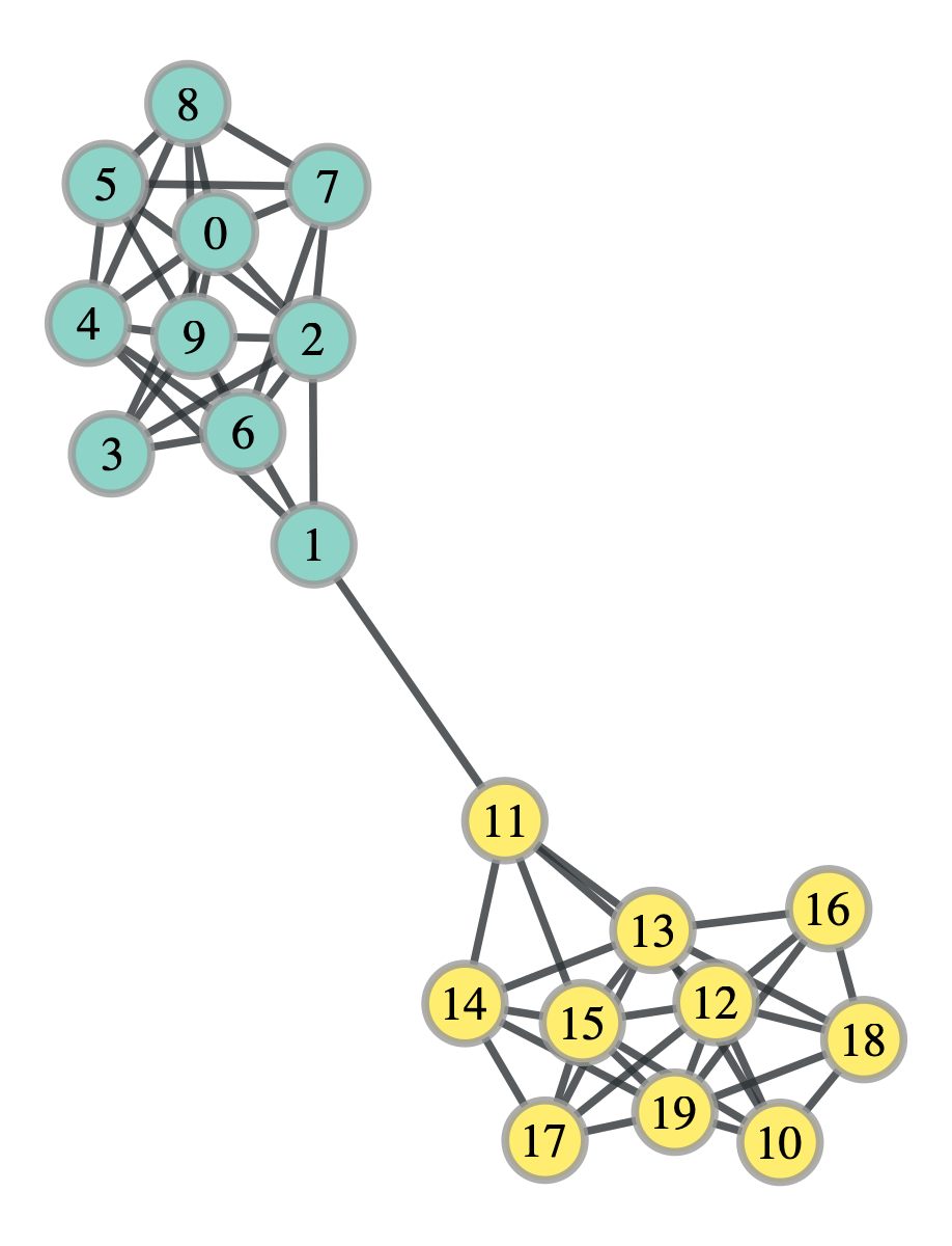 It worked! The colors represent the two groups and we see that it was perfectly divided. Let’s take a look at how the log likelihood changed over the trials
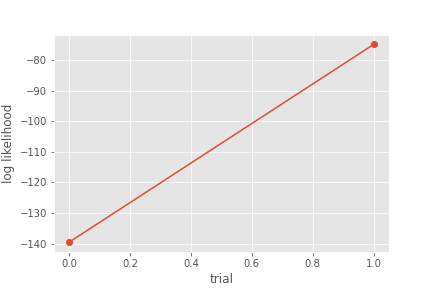 In just two trials, the algorithm was able to find the optimal log likelihood. I am hiding something here, however. It is not guaranteed that the algorithm will find the global maximum. It is totally possible that the algorithm get stuck at a local maximum. What this looks like in terms of the algorithm is that every node move results in a decrease in the likelihood even though it hasn’t yet found the maximum. Indeed if you run the code in the repo, you might find that you have to repeat it several times until the correct division is found, this problem is also discussed in the paper by Karrer and Newman, where they advise running the algorithm multiple times and taking the best run.
Karate Club
The Karate Club network is the first real world example of a network we will touch upon! This is a commonly used network in the literature used to test the performance of novel algorithms, the best part is, it’s included in graph-tool.
k_club_graph = gt.collection.data['karate']
gt.graph_draw(k_club_graph, vertex_text=k_club_graph.vertex_index)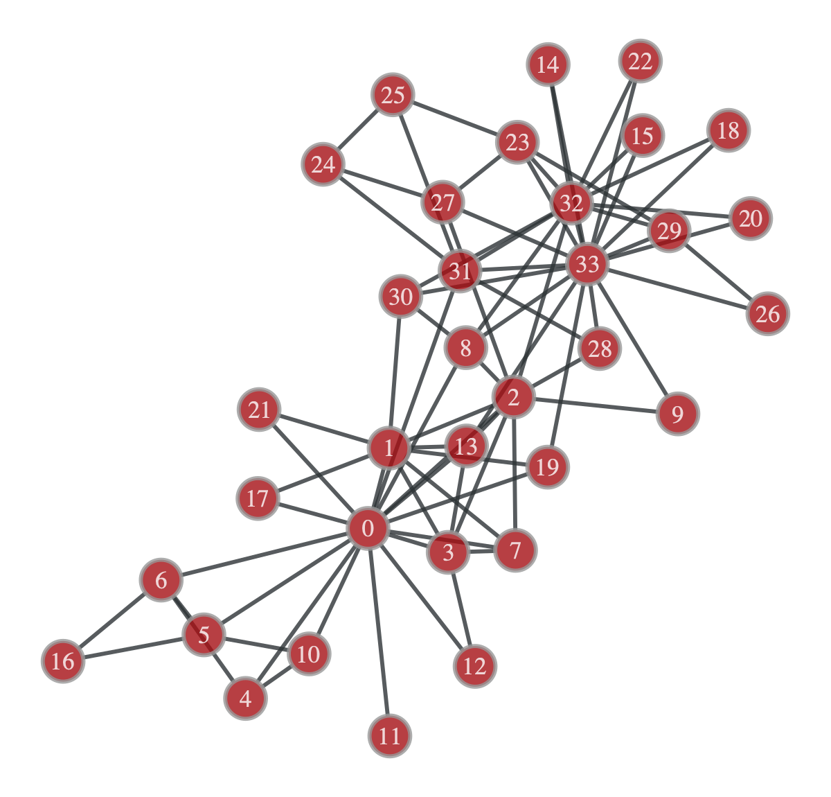 Let’s do some community detection.
k_club = Communities(k_club_graph, 2, model='sbm')
k_club_probs = k_club.get_communities()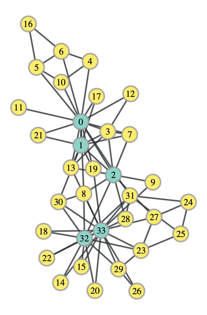 Interestingly, this division does in fact maximize the stochastic block model likelihood, however, it doesn’t look particularly “divided”. Let’s try with the degree corrected stochastic block model
k_club_dc = Communities(k_club_graph, 2, model='dcsbm')
k_club_dc_probs = k_club_dc.get_communities()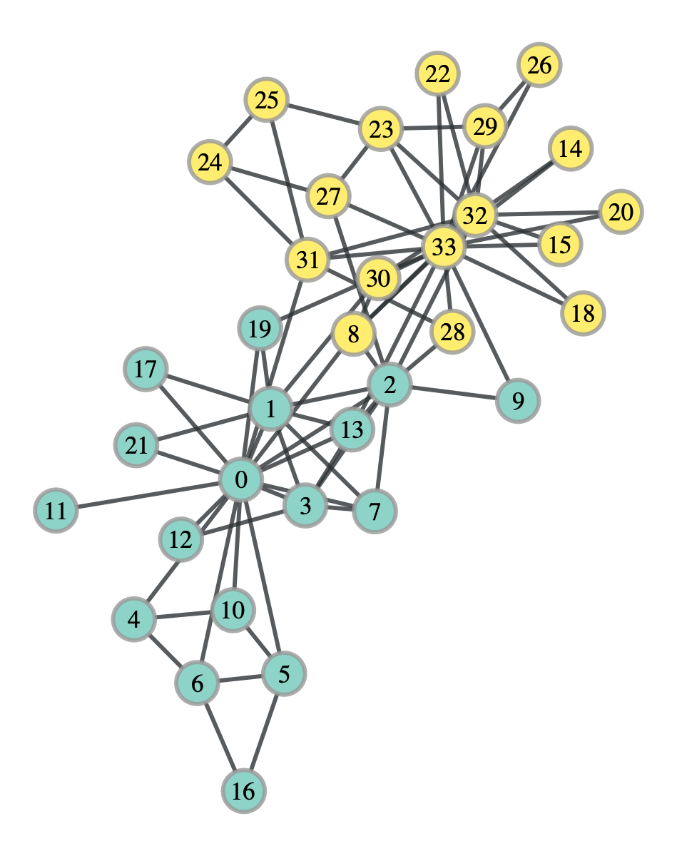 This division looks far more like it. In fact, it isn’t exactly right, but it does match up with what Karrer and Newman got. You may be wondering, which of the two divisions, the standard SBM or the degree corrected version, actually corresponds to the community structure of the network. Well it turns out that it’s the degree corrected version, which matches up with our intuition. However, intuition is not a quantifiable metric, and in general, you will have multiple plausible divisions of a network and it just may be impossible to definitely call one the true division. Peel et al discuss this in depth in their paper, and even give a plausible explanation for the division of the Karate Club network we got using the standard SBM.
Conclusion
The algorithm we used here to maximize the log likelihood is actually just a a heuristic. This means that it’s not guaranteed to find any optima of the log likelihood but it is easy to understand and implement. In fact, this particular implementation is not particularly efficient, there are lots of loops and matrix multiplications that really slow down the code. However, I decided to write it like this so that it matched closely the steps we took in the derivation and keep the algorithm steps as transparent as possible. I implore the reader to find more clever ways to implement this algorithm (Karrer and Newman, for example, optimize the change in likelihood rather than the likelihood itself, this reduces the number of variables that need to be recalculated on each iteration). In a future post I will go over markov monte carlo methods that theoretically sample directly from the distribution we are assuming our networks were draw from.